Agricultural Site Suitability Analysis Using Google Earth Engine and GIS

---

A GIS and Remote Sensing Based Multi-Criteria Decision Analysis (MCDA) Approach

1. Introduction

Agriculture is one of the most important sectors supporting human life, food security, and economic development. Identifying suitable agricultural land is essential for sustainable farming practices, efficient resource management, and increasing agricultural productivity. Traditional land suitability analysis methods are time-consuming and require extensive field surveys. However, advancements in Geographic Information Systems (GIS), Remote Sensing (RS), and cloud computing platforms such as Google Earth Engine (GEE) have significantly improved spatial analysis capabilities.

This project focuses on Agricultural Site Suitability Analysis using Remote Sensing and GIS techniques in Google Earth Engine. The study integrates multiple environmental parameters such as vegetation condition, land surface temperature, and terrain slope using a Weighted Overlay Analysis approach.

The suitability model is developed using:

• NDVI (Normalized Difference Vegetation Index)

• Land Surface Temperature (LST)

• Slope

The analysis is performed using Landsat 8 satellite imagery and SRTM Digital Elevation Model (DEM) data. The final output categorizes the study area into different agricultural suitability zones.

2. Objectives of the Study

The major objectives of this project are:

1. To identify suitable agricultural areas using GIS and Remote Sensing techniques.

2. To generate NDVI, LST, and Slope maps for the study area.

3. To classify environmental parameters into suitability classes.

4. To apply weighted overlay analysis using Multi-Criteria Decision Analysis (MCDA).

5. To produce a final agricultural suitability map.

6. To demonstrate the application of Google Earth Engine for spatial suitability analysis.

7. Study Area

The study area boundary was imported into Google Earth Engine using a user-uploaded shapefile asset. Study area is 28 GP’s of Salekasa Block of Gondia District from Maharashtra.

The Area of Interest (AOI) defines the geographical boundary used for image clipping, analysis, and export.

Fig.: Study Area in Google Earth Engine

5. Data Sources

5.1 Landsat 8 Collection 2 Level 2

Dataset:

LANDSAT/LC08/C02/T1_L2 Source:

United States Geological Survey (USGS) Purpose:

• NDVI generation

• Land Surface Temperature calculation Specifications:

5.2 SRTM DEM

Dataset:

USGS/SRTMGL1_003 Source:

NASA / USGS Purpose:

• Slope generation

• Terrain analysis Specifications:

6. Methodology

The methodology consists of several stages:

1. Data Acquisition

2. Preprocessing

3. NDVI Generation

4. LST Calculation

5. Slope Analysis

6. Reclassification

7. Weighted Overlay Analysis

8. Final Suitability Mapping

9. Data Preprocessing

The Landsat 8 imagery was filtered using:

• Study area boundary

• Date range

• Cloud cover

Code Used

var l8 = ee.ImageCollection("LANDSAT/LC08/C02/T1_L2")

.filterBounds(aoi)

.filterDate("2025-01-01","2025-12-31")

.filter(ee.Filter.lt('CLOUD_COVER',10))

.sort("CLOUD_COVER")

.first();

Purpose

• Remove cloudy images

• Select best quality imagery

• Reduce atmospheric interference

8. NDVI Analysis

8.1 Introduction to NDVI

NDVI (Normalized Difference Vegetation Index) is one of the most widely used vegetation indices in remote sensing. It measures vegetation health and greenness.

Healthy vegetation strongly reflects Near Infrared (NIR) radiation and absorbs Red light.

NDVI Formula

The NDVI (Normalized Difference Vegetation Index) formula is:

NDVI=NIR−Red/NIR+Red Where:

• NIR = Near Infrared Band

• Red = Red Band

For Landsat 8:

• NIR = Band 5 (SR_B5)

• Red = Band 4 (SR_B4)

8.2 NDVI Generation in GEE

var ndvi = l8.normalizedDifference(['SR_B5','SR_B4']) .clip(aoi)

.rename("NDVI");

Fig. NDVI Classification in GEE

9. Land Surface Temperature (LST)

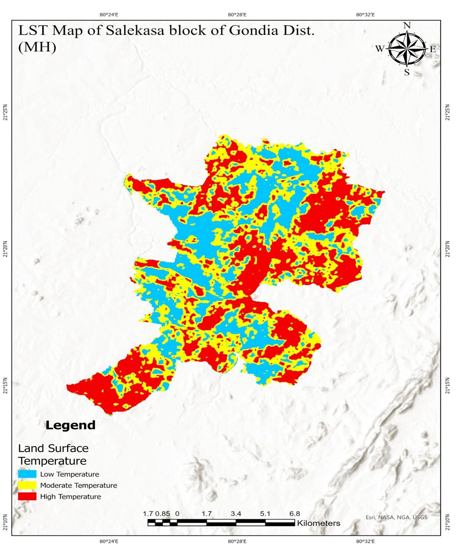
9.1 Introduction to LST

Land Surface Temperature (LST) measures the radiative skin temperature of the Earth’s surface.

In agricultural suitability analysis:

• Lower temperature zones are generally more suitable.

• Higher temperature zones may indicate dry or stressed land.

9.2 LST Calculation

Thermal band ST_B10 from Landsat 8 was used.

Kelvin Conversion Formula

LST K=STB10×0.00341802+149.0 Where:

• LSTK = Land Surface Temperature in Kelvin

• STB10 = Thermal Band 10 value from Landsat 8

• 0.00341802 = Scale factor

• 149.0 = Additive offset

Celsius Conversion Formula

LST C=LSTK−273.15 Where:

• LSTC = Temperature in Celsius

• 273.15 = Conversion constant from Kelvin to Celsius

9.3 LST Code

var st = l8.select("ST_B10");

var lstK = st.multiply(0.00341802)

.add(149.0);

var lstC = lstK.subtract(273.15)

.clip(aoi)

.rename("LST");

9.4 LST Classification

Fig.: Land Surface Temperature (LST) Classification in GEE

10. Slope Analysis

10.1 Introduction to Slope

Slope represents terrain steepness.

Agricultural land is generally more suitable in flatter areas because:

• Easier irrigation

• Lower soil erosion

• Better mechanization

• Improved water retention

Steep slopes are less suitable due to runoff and erosion.

10.2 Slope Generation

Slope was generated using the SRTM DEM.

var dem = ee.Image("USGS/SRTMGL1_003")

.clip(aoi);

var slope = ee.Terrain.slope(dem);

10.3 Slope Classification

Fig.: Slope Classification in GE

11. Reclassification Process

Each thematic layer was reclassified into three suitability classes:

Class Meaning

1. Low Suitability

2. Moderate Suitability

3. High Suitability

Reclassification standardizes different datasets into a common suitability scale.

12. Weighted Overlay Analysis

12.1 Introduction

Weighted Overlay Analysis is a Multi-Criteria Decision Analysis (MCDA) method used in GIS.

Different thematic layers are assigned weights based on their importance.

12.2 Weights Assigned

NDVI was given the highest weight because vegetation health is the primary indicator for agricultural suitability.

12.3 Weighted Overlay Formula

Suitability=(NDVI×0.4)+(Slope×0.3)+(LST×0.3) Where:

• NDVI × 0.4 → Vegetation suitability weight (40%)

• Slope × 0.3 → Terrain suitability weight (30%)

• LST × 0.3 → Temperature suitability weight (30%)

Interpretation

• Higher NDVI increases suitability

• Lower slope increases suitability

• Lower temperature increases suitability

The final weighted value determines:

• Low suitability

• Moderate suitability

• High suitability zones for agriculture.

12.4 Weighted Overlay Code

var ndviWeight = ndviClass.multiply(0.4); var slopeWeight = slopeClass.multiply(0.3); var lstWeight = lstClass.multiply(0.3); var weightedSuitability = ndviWeight .add(slopeWeight)

.add(lstWeight)

.rename("Agri_Suitability");

13. Final Suitability Classification

The final agricultural suitability map was categorized into three classes.

Final Class Suitability Level

1 Low Suitability

2 Moderate Suitability

3 High Suitability

14. Visualization

NDVI Visualization

Fig. NDVI Classification in ArcGIS Pro

LST Visualization

Fig.: Land Surface Temperature (LST) Classification in ArcGIS Pro

Slope Visualization

Fig.: Slope Classification in ArcGIS Pro

Final Suitability Map

Fig.: Final Agriculture Site Suitability in GEE

Fig.: Final Agriculture Site Suitability in ArcGIS Pro

15. Exporting Results

The final suitability map was exported to Google Drive.

Export.image.toDrive({ image: weightedSuitability,

description:"Agricultural_Suitability_Map", folder:'GEE_Output', fileNamePrefix:'Agri_Suitability', region:aoi.geometry(), scale:30, maxPixels:1e13

});

16. Results and Discussion

Interpretation of Final Agricultural Suitability Map

The final Agricultural Site Suitability Map of Salekasa Block, Gondia District (Maharashtra) shows the spatial distribution of agricultural suitability classes across the study area. The map was generated using weighted overlay analysis integrating NDVI, Land Surface Temperature (LST), and Slope parameters.

Observations from the Final Map

1. High suitability zones (green color) dominate most parts of the study area, indicating favorable agricultural conditions.

2. Moderate suitability zones (yellow color) are distributed in patches throughout the central, eastern, and southern portions of the block.

3. Low suitability zones (red color) are very limited and mostly observed along boundary regions and isolated patches.

4. The predominance of high suitability areas suggests that the region has:

   1. Healthy vegetation conditions

   2. Relatively low surface temperature

   3. Gentle terrain slope

5. Moderate suitability areas may represent:

   1. Moderate vegetation cover

   2. Slightly higher thermal stress

   3. Undulating terrain conditions

6. Low suitability regions may be associated with:

   1. Sparse vegetation

   2. Higher land surface temperature

   3. Steeper terrain or degraded land

7. The spatial pattern indicates that Salekasa Block possesses strong agricultural potential and can support extensive agricultural activities with proper land management practices.

8. The map also demonstrates the usefulness of Remote Sensing and GIS-based MCDA techniques for regional agricultural planning and resource assessment.

The final suitability map provides valuable information for:

• Agricultural land-use planning

• Crop management strategies

• Irrigation planning

• Sustainable agriculture development

• Decision-making for resource allocation

17 Results and Discussion

The final agricultural suitability map successfully identified areas with varying agricultural potential.

High Suitability Areas

These regions generally exhibit:

• Healthy vegetation

• Low surface temperature

• Flat terrain

These areas are ideal for:

• Crop cultivation

• Irrigated agriculture

• Intensive farming

Moderate Suitability Areas

These regions show:

• Moderate vegetation

• Moderate terrain slope

• Average temperature conditions

These areas can support agriculture with proper management.

Low Suitability Areas

These regions exhibit:

• Sparse vegetation

• High temperature

• Steep slopes

Such areas may face:

• Soil erosion

• Water stress

• Reduced crop productivity

Applications of Agricultural Suitability Analysis

• Agricultural planning

• Crop suitability assessment

• Irrigation planning

• Sustainable land management

• Precision agriculture

• Resource optimization

• Government agricultural schemes

Conclusion

This study demonstrated the application of Google Earth Engine for agricultural suitability analysis using Remote Sensing and GIS techniques. The integration of NDVI, Land Surface Temperature, and Slope through Weighted Overlay Analysis successfully identified suitable agricultural zones.

The study highlights the effectiveness of cloud-based geospatial analysis platforms for land suitability assessment. The methodology is simple, efficient, scalable, and suitable for regional agricultural planning.

The generated suitability map can assist planners, researchers, and policymakers in sustainable agricultural development and resource management.

---

References

1. Agricultural land use suitability analysis using GIS and AHP technique Halil Aknc , Ayse Yavuz Özalp1, B lent Turgut (Google Scholar)

2. USGS Landsat 8 Collection 2 Level 2 Dataset

3. NASA SRTM Digital Elevation Model

4. Google Earth Engine Documentation

5. FAO Land Suitability Evaluation Guidelines

6. Jensen, J.R. (2005). Introductory Digital Image Processing.

7. Lillesand, T., Kiefer, R., & Chipman, J. (Remote Sensing and Image Interpretation)

8. Burrough, P.A. and McDonnell, R.A. (Principles of GIS)

9. Eastman, J.R. Multi-Criteria Evaluation and GIS

10. Remote Sensing Applications in Agriculture Research Papers

11. GIS-Based Agricultural Land Suitability Analysis Studies

---

Appendix: Complete GEE Code

var aoi = ee.FeatureCollection(

'projects/future-yeti-494405-s4/assets/AOI'

);

Map.centerObject(aoi, 10);

Map.addLayer(aoi,

{color:'red'},

'Study Area');

var l8 = ee.ImageCollection("LANDSAT/LC08/C02/T1_L2")

.filterBounds(aoi)

.filterDate("2025-01-01","2025-12-31")

.filter(ee.Filter.lt('CLOUD_COVER',10))

.sort("CLOUD_COVER")

.first();

var st = l8.select("ST_B10");

var lstK = st.multiply(0.00341802)

.add(149.0);

var lstC = lstK.subtract(273.15)

.clip(aoi) .rename("LST");

var ndvi = l8.normalizedDifference(['SR_B5','SR_B4'])

.clip(aoi)

.rename("NDVI");

var dem = ee.Image("USGS/SRTMGL1_003")

.clip(aoi);

var slope = ee.Terrain.slope(dem);

var ndviClass = ee.Image(0).clip(aoi)

.where(ndvi.lte(0.2), 1)

.where(ndvi.gt(0.2)

.and(ndvi.lte(0.5)), 2)

.where(ndvi.gt(0.5), 3);

var lstClass = ee.Image(0).clip(aoi)

.where(lstC.lte(25), 3)

.where(lstC.gt(25)

.and(lstC.lte(35)), 2)

.where(lstC.gt(35), 1);

var slopeClass = ee.Image(0).clip(aoi)

.where(slope.lte(5), 3) .where(slope.gt(5)

.and(slope.lte(15)), 2)

.where(slope.gt(15), 1);

var ndviWeight = ndviClass.multiply(0.4); var slopeWeight = slopeClass.multiply(0.3); var lstWeight = lstClass.multiply(0.3);

var weightedSuitability = ndviWeight .add(slopeWeight)

.add(lstWeight)

.rename("Agri_Suitability");

var suitabilityVis = { min:1, max:3,

palette:['red','yellow','green']

};

Map.addLayer( weightedSuitability, suitabilityVis,

"Agricultural Suitability"

);

Export.image.toDrive({ image: weightedSuitability,

description:"Agricultural_Suitability_Map", folder:'GEE_Output', fileNamePrefix:'Agri_Suitability', region:aoi.geometry(), scale:30, maxPixels:1e13

});

print("Agricultural Suitability Analysis Completed");