
.png)

Introduction & Objective:
Accurate assessment and mapping of building density are critical components in the toolkit of modern urban planning, sustainable development, and environmental management. In rapidly growing metropolitan environments, such as Bengaluru Urban district in Karnataka, India, the ability to quantify and analyse the spatial distribution of built-up structures underpins effective infrastructure design, disaster resilience planning, service delivery, and smart city governance.
Traditional approaches relying on census data, administrative boundaries, or manual land-use surveys can be limiting due to scale, temporal lag, and lack of granularity. The evolution of open building footprint datasets, such as those provided by Google and Microsoft, paired with cloud-based geospatial analysis environments like Google Earth Engine (GEE) and advanced visualization platforms like QGIS, enables highly scalable, reproducible, and fine-grained building density mapping workflows that address contemporary urban challenges.
This methodology report is designed to empower GIS professionals, city planners, researchers, and policymakers through a structured, end-to-end workflow for spatial building density analysis. The process begins with the rigorous and precise definition of the study area using authoritative administrative boundary datasets (FAO GAUL Level-2), ensuring that all subsequent spatial analyses are contextually relevant and statistically robust. By leveraging global AI-generated building footprint collections, the workflow overcomes traditional biases and data gaps, extending coverage even to fast-changing or informal urban zones.
The report details the construction of spatial grids (e.g., 1000m x 1000m) within the target region for systematic sampling and density calculation. Integration of these grids with high-resolution building polygon data via efficient spatial joins in Earth Engine allows calculation of both the number and total area of built structures per grid cell, enabling refined zonal or neighborhood-level metrics. The resulting spatial datasets are exported and interrogated within QGIS, where advanced cartography and thematic mapping techniques are used to produce actionable visualizations and support multi-scale decision support.
Key objectives of this methodology include:
-
Providing a repeatable and scalable framework for urban building density analysis adaptable to diverse global contexts and data sources.
-
Maximizing data quality, coverage, and consistency by utilizing validated open datasets and robust data cleaning/geoprocessing practices.
-
Enabling multi-resolution analysis and reporting—from grid cell-based summaries to administrative zone or ward-level aggregation.
-
Supporting future extensions for time-series analysis, risk assessment, urban health studies, infrastructure investment, and citizen engagement.
By detailing each process, potential pitfalls, and solutions, this methodology lays a foundation for transparent, data-driven urban governance and spatial research. It facilitates collaboration across disciplines and institutions while enabling continual updates and improvements to urban spatial intelligence as new datasets and tools become available.
Study Area Definition:
The first step is precise study area selection.
-
The FAO GAUL Level-2 administrative boundaries provide district-level polygons globally.
-
Here, the Bengaluru Urban district in Karnataka, India is selected by filtering for the country (ADM0_NAME = "India"), state (ADM1_NAME = "Karnataka"), and district (ADM2_NAME = "Bangalore Urban").
-
The boundary is visualized in the GEE code editor to confirm correct spatial focus.
-
This geometry will constrain all subsequent data queries and processing, ensuring relevance and computational efficiency.
Open Building Footprint Dataset Acquisition (Data Source):
Two authoritative open datasets are referenced:
-
Google Open Buildings v3: Derived from high-resolution satellite imagery using advanced ML, this vector dataset provides up-to-date building polygons for most regions.
-
Microsoft Global Building Footprints: A nationwide (including India) ML-extracted building polygon resource, useful for alternative or combined analysis.
-
The chosen dataset is loaded as an ee.FeatureCollection and then filtered (filterBounds) using the study area's geometry to retain only features within the target district.
This produces a baseline layer of all buildings relevant to the analysis area.
Grid Generation for Zonal Mapping
-
A regular grid of specified size (e.g., 1000m x 1000m) is generated using the geometry.coveringGrid() function in GEE.
-
The grid uses a projected CRS (such as EPSG:32643 for southern India UTM zone) to ensure equal-area cells, critical for density analysis.
-
The grid is visualized in the GEE map to confirm alignment and coverage.
-
This transforms the continuous study region into a set of systematic, comparable spatial units—preparing for grid-based analytics
Spatial Join and Aggregation in GEE
-
For each grid cell, a spatial join using ee.Join.saveAll and ee.Filter.intersects attaches all building polygons that intersect the cell.
-
The join produces a new collection, where each grid cell's attributes now include a list of overlapping buildings.
-
This join enables fast, scalable aggregation for per-cell statistics.
Calculation of Per-Grid Building Metrics
-
For each grid cell:
-
Building Count: The length of the attached building list reflects the number of buildings in that cell.
-
Total Built-Up Area: Areas of each intersecting building are calculated and then summed per cell using a reducer such as ee.Reducer.sum.
-
Both metrics are stored as attributes (total_buildings, total_area) for each grid polygon.
-
-
The result is a fine-grained spatial database capturing both the number and total area of buildings in every grid cell, ready for export and further analysis.
Export from Earth Engine and Preparation for QGIS
-
Use GEE’s Export.table.toDrive() function to save the enriched grid as a shapefile, including building count and area fields.
-
Download the resulting shapefile (grid_with_building_area.shp) to your local system.
-
Inspect in QGIS (or other GIS) to ensure all grid cells and attributes are present and consistent.
Advanced Spatial Analysis and Clipping in QGIS
-
Add both the building grid shapefile and the relevant administrative or zone boundary layer (e.g., BBMP zones, city wards) to QGIS.
-
Both layers share the same coordinate system (reproject as necessary).
-
Use QGIS “Clip” or “Intersection” (Vector Overlay tools) to restrict grid data to the exact shape of each zone or ward:
-
If your analysis needs purely zone-based (not grid-based) summarization, use “Join Attributes by Location” (with ‘contains’ or ‘intersects’ logic) to associate each grid cell’s attributes with the containing zone.
-
For additional statistics (sum, mean, density per zone), use “Group Stats” or similar methods to aggregate as needed.
-
Thematic Mapping and Visualization in QGIS
-
Open the zone/grid layer properties. In “Symbology,” select “Graduated” style using building count or density as the target field.
-
Define bins and color ramps to mirror established density mapping conventions (e.g., 1–100, 100–500, etc., per sq km).
-
Adjust classes and palette for clarity and interpretability, adding context basemaps (OpenStreetMap, satellite imagery) as desired.
-
Design the map layout with legends, title, scale, and north arrow in QGIS “Print Layout.”
Final Map Export, Applications, and Extensions
-
Export the final map product as PNG or PDF for use in reports, presentations, or web dashboards.
-
The resulting map enables:
-
Data-driven urban planning and infrastructure optimization.
-
Disaster risk analysis (e.g., fire, flood) in high-density grids.
-
Smart city management through zone-wise resource allocation.
-
Longitudinal studies by repeating the workflow with updated or time-stamped building data.
-
OUTPUT :
Zone wise map for Bengaluru using Qgis Map Layout

Bommanahalli
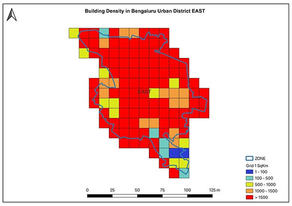
East Zone

MAHADEVAPURA ZONE

RR NAGARA ZONE

SOUTH ZONE

WEST ZONE

YELAHANKA ZONE

Screenshort from Google Earth Engine

Screen Shot from Google Earth Engine with Building polygons
Conclusion
This comprehensive methodology establishes a robust foundation for building density mapping in urban analytics, integrating global open building datasets, Google Earth Engine for large-scale spatial computing, and QGIS for advanced visualization and cartographic output. The systematic workflow—beginning with high-precision study area selection, followed by rigorous data acquisition, cleaning, grid generation, spatial joining, and culminating in thematic mapping—ensures reproducibility, scalability, and practical utility for urban management, infrastructure planning, and policy development. The project not only demonstrates the technical feasibility of detailed building density analysis at grid and zone levels but also highlights how these results empower stakeholders with actionable spatial intelligence for optimized resource allocation and informed decision-making.